
OVERVIEW
This project addresses the complex geospatial modeling challenge presented by Project Skydrop, a real-world treasure hunt requiring the discovery of a hidden prize using clues.
By leveraging data clues taken from the hidden location and conditioning global context from satellites, we reason about the relative likelihood of the treasure’s position across a shrinking search grid. We formulate this search as a sequential estimation problem, utilizing a Hidden Markov Model (HMM) to iteratively update our belief state. The technical approach moves beyond naive baselines to employ Multimodal Variational Autoencoders (VAEs) and Flow Matching for precise likelihood estimation, while prioritizing calibrated uncertainty through MultiSWAG to ensure robust predictions in a unique low-data regime.

- INTRODUCTION
- DATA: SOURCES
- DATA: MOTIVATING EXAMPLE
- DATA: COLLECTION
- CONFIDENCE IN PREDICTIONS
- METHOD: HMM
- METHOD: NAIVE LIKELIHOOD ESTIMATION
- METHOD: ESTIMATING LIKELIHOOD
- VAE: BASICS
- VAE: OPTIMIZATION
- VAE: ALIGNMENT OF MODALITIES
- FLOW MATCHING: BASICS
- FLOW MATCHING: CONDITIONAL LIKELIHOOD
- MODELING EPISTEMIC UNCERTAINTY
- INTERESTING RELATION TO AUDIO PROCESSING
- CONCLUSION
INTRODUCTION
Project Skydrop is a real-world treasure hunt that challenges participants to locate a hidden prize through a series of gradually refined clues. The game unfolds by initially providing a large shrinking circle over a geographical area that includes the possible location of the treasure. As the event progresses, clues from the hidden location are released daily, each narrowing the search area until the prize’s location is ultimately revealed.
The treasure, a 4-inch-tall 24-karat gold statuette weighing 10 troy ounces, was valued at more than 30,000 dollars. Additionally, a prize bounty was collected with the entry fee of each new participant joining the hunt. By the time the treasure was found the total prize pool was over 115,000 dollars.
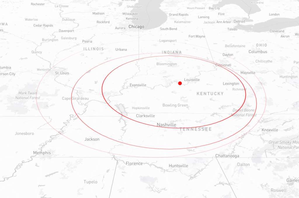

The event attracted treasure hunters nationwide, culminating in the discovery of the treasure in Wendell State Forest, Massachusetts, by a Boston meteorologist who used weather patterns to identify the location. The unique real world formulation of the hunt as well as the data driven method in which the treasure was found, presents a challenging geospatial modeling problem which this project aims to address. We seek to construct a model capable of effectively localizing a hidden location across a wide variety of geographical and meteorological conditions, in the shortest amount of time possible.
DATA: SOURCES
There are two main sources of data that would be useful for this goal of localizing the treasure. The first source is clues directly from the unknown geographical location of the treasure. In the case of this specific treasure hunt, it is given through a trail camera overlooking the treasure.
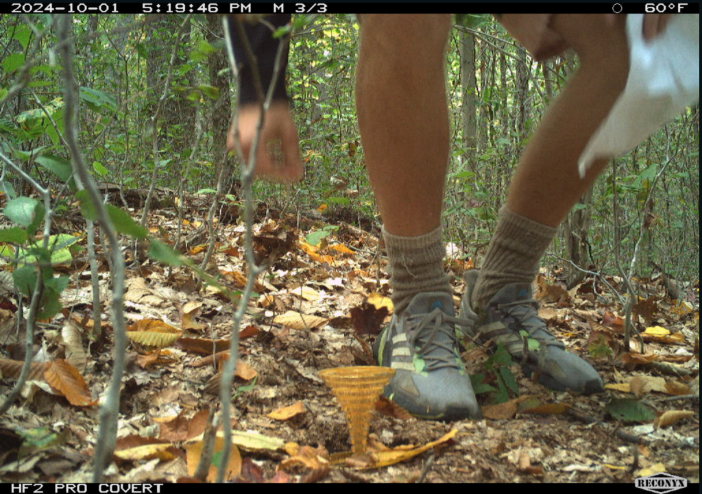
Trail Camera Imagery: A trail camera overlooking the treasure captures images every 15 minutes (up to 96 images per day). These images provide environmental monitoring, offering clues such as.
- Cloud Cover and Lighting Variations: Changes in brightness may indicate cloud density and weather shifts.
- Precipitation and Sundown Effects: Variations in lighting and weather can hint at atmospheric conditions and location.
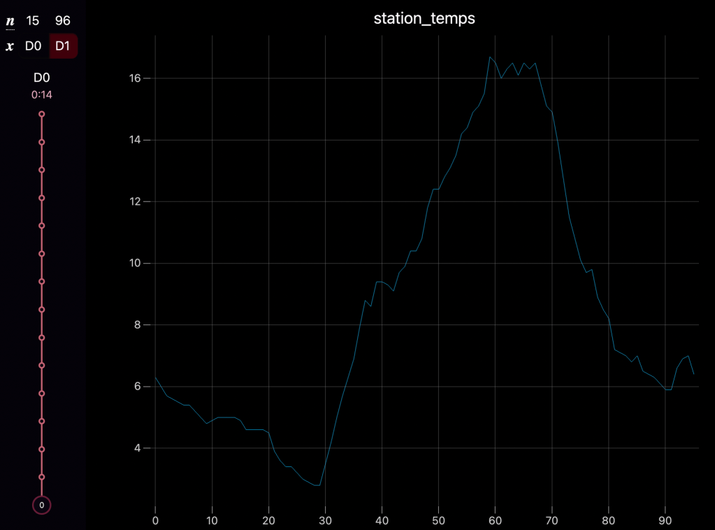
- Temperature Readings: Temperature data from the camera can be used to detect spikes or notable features in weather patterns of the area.
The second source of useful data would be anything covering the geographical search area of possible hidden locations that tells you something useful about the underlying environment. You can then compare this data with the location specific data to reason about relative probabilities of where the hidden location is.
DATA: MOTIVATING EXAMPLE
Situation: Lets say the underlying meteorological condition for a specific day is that there is a cold front sweeping through the search area. Since the hidden location’s data is dependent on this underlying environment condition, it is likely that some data from the location reflects these conditions. For example the temperature data may pick up on the cold front and registers a sudden drop in temperature at a specific time during the day.
Problem: By its self this data isn’t particularly useful in finding the hidden location, as there is nothing for it to compare against.
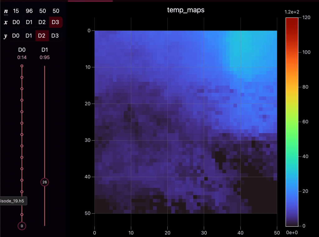
Solution: But if we introduce the second source of data such as a global satellite temperature map over the search area, then it becomes possible to compare this location specific data to the global one. By interpreting patterns in the global temperature map it’s possible to find what locations experience this sudden drop in temperature and reason about relative likelihoods of where the treasure may be hidden.
The goal of this project is to create a machine learning model flexible enough to take in these multimodal location specific clues, as well as multimodal global search area data and reason about the relative likelihoods of locations containing the hidden treasure, uncovering these complex patterns between the two sources automatically.
For the evaluation of this method I chose to focus on the two modalities discussed in the motivating example above: local temperature readings from the hidden location and global satellite temperature maps over the search area.
While focusing on these modalities for now, the machine learning model was designed to be able to easily expand and support others like wind or precipitation, in both the local location and global map. The key is that the network learns to use the modality specific data to reason about what the underlying environmental condition that data describes. Then this predicted underlying condition is used to reason about it’s likelihood under conditions across the global search area. In this way the likelihood model is constructed to be modality independent.
DATA: COLLECTION
The development of an effective model for localizing the treasure in Project Skydrop relies heavily on the acquisition and careful preparation of relevant data over a wide range of geographical conditions.
Given the impracticality of manually collecting trail camera temperature data across a multitude of locations and conditions, we will employ a simulation approach using historical data from personal weather stations (PWS) available on the Weather Underground website. By scraping the website’s data from various PWS locations, we can create a training dataset that reflects a wide range of potential treasure locations and their corresponding temperature profiles.
To obtain the necessary satellite-based temperature maps for our training dataset, we will utilize the Open Meteo API. Their Historical Weather API is based on reanalysis datasets that integrate various observational sources, including satellite data, with weather models to create a comprehensive and consistent record of past weather conditions. We can query this API using specific geographical coordinates (corresponding to the centers of our grid cells) and date ranges to retrieve the temperature data needed to construct our 24-hour temperature maps at 15-minute intervals for our chosen training locations.
Unfortunately Open Meteo has an API limit request and the Weather Underground Website makes it difficult to automate the selection of stations to scrape data from. Both of these issues result in a unique low data challenge for training the model, which motives some of my design choices.
CONFIDENCE IN PREDICTIONS
Before diving into the specific methods that I have explored and eventually settled on, I want to mention some important considerations to make in terms of what it means to have calibrated confidence in our predictions.
A critical aspect of the Skydrop Predictor is its ability to output well-calibrated probability estimates for the treasure’s location. Ideally, if the model assigns a 25% probability to a particular area, then in roughly one-forth of cases where similar conditions exist, the treasure should indeed be found within that area. Achieving such calibration requires careful consideration of two main types of uncertainty.
Epistemic Uncertainty
This uncertainty reflects limitations in the model’s knowledge, stemming from sparse or incomplete data within the training distribution and is often reducible by incorporating additional training data. In situations with sparse data it is often beneficial to reason about the uncertainty in choice of model weights, instead of picking the best point estimate in typical optimization methods
Aleatoric Uncertainty
This is the irreducible uncertainty inherent in the data itself (e.g., measurement noise, environmental variability). It represents the natural randomness of the observational process, and can be reasoned about by adjusting the model’s output. The uncertainty is homoscedastic when the input does not effect the model’s output confidence, and can be accounted for by tuning output probabilities with temperature scaling. On the other hand the uncertainty is heteroscedastic when the confidence varies with the input, and is mitigated by including a mean and measure of confidence in the model’s output. In situations where the data is noisy and the model can’t make a good prediction, it can learn to decrease the loss by increasing its own uncertainty.
METHOD: HMM
The challenge of locating a hidden prize through a series of progressively refined clues presents a compelling problem in sequential estimation. One potential approach is to train a neural network to process all available data at once and output a probability distribution over the grid space. However, generalizing such a model would require an extensive dataset to capture the complexity of temperature variations over long time sequences.
Instead, by framing the problem as a Bayesian filtering task, we can incorporate new evidence incrementally each day, fixing the sequence length, and making data collection more feasible.
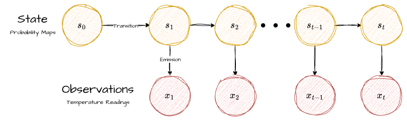
This naturally leads to the formulation of a hidden Markov model (HMM), where clues serve as observable events influenced by an unobserved hidden state, the location of the treasure. Although the Markov assumption reduces expressiveness by restricting dependencies to only the previous state, this tradeoff improves the efficiency, structure, and interpretability of the data. HMMs offer a clear probabilistic framework, making it possible to manually incorporate human biases and domain knowledge into the predictive model as the treasure hunt progresses. Each day’s posterior distribution becomes the prior for the next, enabling continuous refinement of the location estimate as new information arrives.
Under the HMM formulation the update rule to incorporate new observations into the posterior distribution each day is with Bayes’ rule.
Since we only care about relative probabilities across the search area we can drop the denominator and the update rule becomes:
The key term we are trying to compute with the network is the likelihood of seeing observations from a location in the search area, given some global context data:
Hidden States
In our model, the hidden states are the possible locations of the treasure within the initial search area. To facilitate computational modeling, this continuous area will be discretized into a grid of cells.
Initial State Distribution
This represents our belief about the hidden state at the beginning of the process. We will use a uniform prior probability distribution across all the grid cells contained within this initial area. This means that at the start, every location within the circle is considered equally likely to hold the treasure.
Transition Probabilities
In a typical HMM, transition probabilities govern the movement between hidden states over time. However, in the context of Project Skydrop, the treasure’s location is fixed. The “transition” in our model refers to the change in our belief about the possible locations due to the shrinking search circle. Each day, the probability of the treasure being in any location outside the current circle becomes zero. This can be viewed as a deterministic transition in the set of plausible hidden states.
Emission Probabilities
Emission probabilities define the likelihood of observing a particular clue given a specific hidden state (conditioned on the global environment data across the grid). We will employ a deep neural network to learn and estimate this likelihood function, as the relationship between temperature patterns and location can be complex.
METHOD: NAIVE LIKELIHOOD ESTIMATION
There are 3 main considerations that influence the design choices for this likelihood estimation model:
- Accurate confidence in predictions
- Limited data for training
- Scalability of method
At first, to explore my data and feasibility of the HMM, I used naive methods of estimating this likelihood via a simple cosine similarity between the temperature from the hidden station and the satellite map. Areas that had similar temperatures would light up and register as higher likelihood. While this method was very data efficient (does not require training), it didn’t preform well in regards to the other aspects of what I was looking for:
- This gives rough likelihood estimates, but the results were not very discriminative or grounded in probabilistic meaning, resulting in inaccurate predictions. For example over a given area in the summer most of the temperature across the grid was very similar, while there were small patterns that could have been picked up by a model, these small patterns don’t register as something meaningful in the cosine similarity metric.
- Additionally, this method doesn’t scale very well to multiple modalities. In particular cross modality likelihoods would not be able to be done, because cosine similarity needs the data to exist in the same dimension and data space. Even within the temperature data, small differences in weather station/satellite sensors resulted in surprisingly different temperature readings for the same geographical location, which wouldn’t show up well in the cosine similarity likelihood estimate.

METHOD: ESTIMATING LIKELIHOOD
There are multiple methods to actually estimating this likelihood in a way that is probabilistically grounded and uses a neural network that can uncover these hard patterns.
Probabilistic Regression (Baseline): Takes in the grid location and conditioning satellite temperature map and predicts a gaussian mean and variance for the expected station temperature. Maximum likelihood estimation is used under this predicted gaussian.
- Benefits: Simple and stable to optimize.
- Drawbacks: Makes a gaussian assumption and assumes uni-modal distribution.
Mixture Density Networks: Takes in the grid location and conditioning satellite temperature map and predicts and set of parameters for multiple gaussians. Maximum likelihood estimation under this mixture of gaussians.
- Benefits: Simple and can capture multi modal distributions.
- Drawbacks: Can be unstable to optimize and still makes gaussian assumption with set number of gaussians.
Normalizing Flows: A network learns a sequence of invertible transformations that map the complex distribution of your data, given the global satellite conditioning, into a more simple gaussian distribution.
- Benefits: Exact computation of likelihood and highly calibrated.
- Drawbacks: Requires invertible network layers which severely limits architecture.
Diffusion Models / Flow Matching (ODE-based): Takes in the grid location and conditioning satellite temperature map and learns a continuous time-dependent vector field. Exact likelihood is computed by numerically integrating an Ordinary Differential Equation (ODE) that traces the path from the data point back to a simple noise distribution.
- Benefits: Can model highly complex distributions without the strict architectural constraints of normalizing flows. Relatively stable to optimize.
- Drawbacks: Extremely slow likelihood evaluation as it requires running the network many times to solve the integral for a single point.
All of these likelihood evaluation methods are by default done in the original station data space, since we are evaluating the likelihood of this station data appearing given the location and global context conditioning.
While for lower dimensional data this may work fine, in high dimensional spaces this likelihood evaluation typically grows unstable. Since we are designing the neural network for multiple modalities, the data space can grow really quick. Additionally as the conditioning variables grow more complex (like spatiotemporal temperature maps) many of these methods are data hungry and require large datasets to not overfit to your training data.
For these reasons I first choose to embed the different modalities and global conditioning data into a smaller shared latent space using a multimodal VAE. By then computing likelihoods in this compressed space, we can achieve more stable training and accurate results under our low data regime.
VAE: BASICS
The primary goal of a standard autoencoder is to learn a compressed representation of your data by training a network to ignore uninformative information. The model works by compressing the input data down into a low dimensional bottleneck and then trying to reconstruct the original input from that compressed vector. While this is effective for simple dimensionality reduction it creates a fragmented latent space with gaps. If you try to sample from or work with latent data in these gaps the information within these codes are often garbage.
The Variational Autoencoder (VAE) solves this by enforcing structure on that latent space. Instead of encoding the input to a single fixed point the VAE encodes it to a probability distribution, typically a gaussian. This forces the model to fill in the gaps and creates a smooth continuous space where similar data points are clustered together. The loss function to achieve this is composed of two competing terms. The reconstruction loss encourages the model to be accurate while the KL divergence term acts as a regularizer that forces the latent distribution to look like a standard gaussian.
VAE: OPTIMIZATION
Training a vanilla VAE often presents significant stability challenges. The main difficulty lies in balancing the two terms of the loss function: the reconstruction error and the KL divergence. If the regularization is too strong, the model suffers from posterior collapse, where the decoder ignores the latent code entirely and just predicts the average of the dataset. This means the mutual information between the input and the latent variable drops to near zero, and the model fails to learn a meaningful latent space. Conversely, if the reconstruction term dominates, the model ignores the prior, leading to good reconstructions but poor generation capabilities and a non-smooth latent space.
Mathematically, this imbalance stems from an implicit assumption in the standard Mean Squared Error (MSE) reconstruction objective. Using a simple MSE loss is equivalent to assuming the decoder is a Gaussian distribution with a fixed, unit variance. This arbitrary assumption fails to account for the model’s actual uncertainty.
In practice, the raw MSE magnitude can vary wildly depending on the data scaling, often overpowering the delicate KL divergence term by orders of magnitude. Without a calibrated variance to normalize this error, the optimization landscape becomes dominated by reconstruction gradients, forcing the model into a rigid trade-off that ignores the prior. To fix this, we look at the true log-likelihood of a Gaussian decoder, which explicitly includes the variance as a weighting factor:
To solve the balancing act without extensive hyperparameter tuning, I utilized the Sigma-VAE formulation. Instead of treating the variance as a fixed constant, the Sigma-VAE treats it as a parameter that needs to be learned. However, rather than learning it via slow gradient descent, we can solve for the optimal variance analytically for every single batch. It turns out that the optimal variance that maximizes the likelihood for a given batch is simply the Mean Squared Error (MSE) of that batch:
By substituting this optimal variance back into the log-likelihood equation, the training objective simplifies elegantly. The explicit MSE term effectively becomes a constant, and the gradients flow primarily through the logarithmic variance penalty. This transforms the reconstruction loss from a linear MSE term into a logarithmic one:
This logarithmic form is the key to the method’s stability. When the model is performing poorly (high MSE), the gradient of the log function is small, preventing the reconstruction loss from overwhelming the KL term and causing posterior collapse. As the model improves and MSE drops, the gradients naturally increase, forcing the model to fight harder for fine-grained details.
This allows the model to dynamically calibrate the weight of the reconstruction loss against the KL divergence. The result is a model that consistently learns high-quality representations and maintains high mutual information without the training instability of the standard approach.
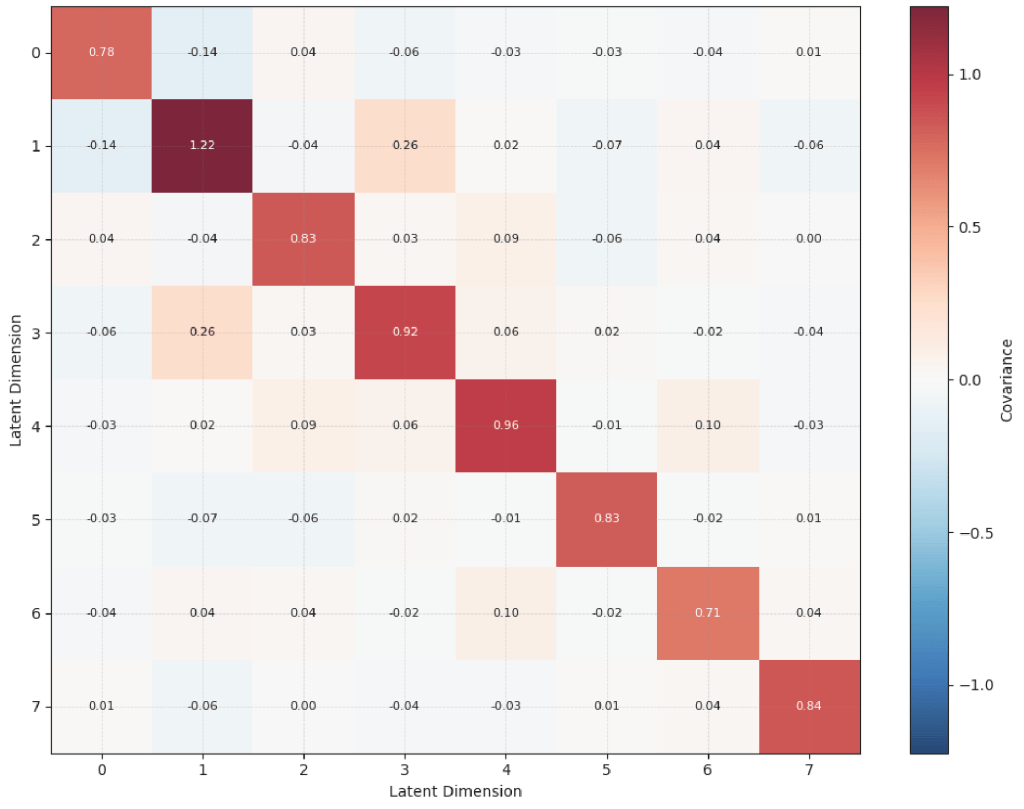
To further refine the representation I added a decorrelation loss to the training objective. Standard VAEs often suffer from redundancy where multiple latent dimensions encode the same information or some dimensions are ignored entirely. By penalizing the covariance between latent dimensions I forced the model to spread the information across the entire latent space. Without this I would often see certain directions in the latent space collapse and become unused, with the model getting stuck in a local optimum of focusing on easy features and failing to learn as meaningful of a latent space. This creates a disentangled space where every dimension is statistically independent and easier to use.
VAE: ALIGNMENT OF MODALITIES
Since our goal is to support multiple station and global context modalities we need all data types that describe the same underlying geospatial condition to exist in the same shared latent space. A common method to achieve this is contrastive learning, similar to how models like CLIP work. This approach aligns modalities by pushing the embeddings of paired data points together while pushing unpaired points apart. While this is powerful for retrieval tasks it does not inherently define how to combine the probability distributions of multiple inputs and breaks probabilistic meaning in the resulting latent distribution.
For this project I settled on a Product of Experts (PoE) formulation. Instead of just aligning the vectors this method mathematically combines the distributions predicted by each modality. If the temperature data predicts a broad area of possible environment conditions, but the wind data confidently predicts a specific condition the product of experts multiplies these densities to find the area of agreement. This results in a sharper and more precise posterior distribution that naturally handles missing or unconfident data. If one modality is noisy or missing, the model naturally relies more heavily on the confident expert.
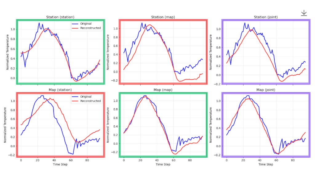
In green you see reconstructions for a modality, coming from its own embedding (good reconstructions). In red you see reconstructions coming from the opposite modality embedding (slightly worse reconstructions, but it is clear it knows the underlying condition). In purple you see the reconstructions made from the joint latent code.
I designed the architecture with separate encoders and decoders for each individual modality. The key to making them share a latent space is in how they are trained. We don’t just encode/decode each modality separately. Instead the model is forced to reconstruct every modality using the latent codes from every other modality plus the joint product code.
This forces the encoders to do more than just compress the input data. For the satellite data encoder to produce a code that can successfully reconstruct the station temperature it has to look past the raw time series. It effectively learns to infer the underlying environmental condition that caused those values to appear. By predicting the physical state of the environment rather than just the features of one modality the encoders naturally align their representations.
This setup is much more data efficient for our low data regime. Since every modality learns from every other modality we get a robust model where a standard feature extractor separately processing information would just overfit. We aren’t just learning features we are learning the shared conditions that generate those features.
FLOW MATCHING: BASICS
Most generative models like diffusion work by slowly removing noise from a signal. While effective standard diffusion is stochastic meaning the path from noise to data is random and jittery. Flow Matching takes a different approach. Instead of learning to remove noise step by step it learns a velocity vector field that pushes a probability distribution directly from simple noise to your complex data. The model in this framework essentially acts like a compass pointing you towards higher density in the data space.
Think of it as defining a smooth continuous flow rather than a series of random jumps. The model learns to predict the direction and speed the data should move at any point in time to transform from a gaussian into the target distribution. This results in straight deterministic paths during generation which are much more efficient and stable than the winding paths of standard diffusion.
FLOW MATCHING: CONDITIONAL LIKELIHOOD
For my hidden treasure problem I need to know the exact likelihood of a specific sensor reading given the satellite context. We can achieve this by conditioning the vector field on the global satellite map and the grid location. This changes the flow so that the path from noise to data is guided by the environment.
The conditioning data, which is the global temperature satellite data is first encoded into a latent map, which is then used as conditioning signal. This allows for more stable training under the low data regime rather than passing in the raw spatiotemporal temperature map which would be prone to overfitting.
To get the likelihood we use the Probability Flow ODE. Instead of generating data we take our observation and solve the ODE backwards in time pushing it back to the noise distribution. As we integrate along this path we calculate the change in density. This gives us the exact log likelihood of that specific reading occurring at that specific location. It is computationally expensive but yields the precise calibrated probabilities required for the HMM update.
MODELING EPISTEMIC UNCERTAINTY
Traditional deep learning architectures operate with a fixed set of weights and biases. These networks undergo a training process where a single optimal value is learned for each parameter, aiming to maximize the likelihood of the provided training data. In contrast, Bayesian neural networks (BNNs) adopt a probabilistic perspective, treating their weights and biases not as fixed values, but as probability distributions. This fundamental shift from single-point estimates to distributions is crucial as it allows BNNs to inherently capture the uncertainty associated with the model’s parameters, thereby directly addressing epistemic uncertainty. When the available data is insufficient to definitively determine the ideal weight value, the resulting posterior distribution for that weight will exhibit a higher variance, reflecting this lack of certainty.
This distribution over the model’s weights given the dataset , embodies the updated beliefs about the weights after considering the information provided by the data and can be expressed as:
We can then use the uncertainty of the model’s weights in this distribution to reason about the uncertainty of the model’s prediction. In Bayesian Model Averaging (BMA) we weigh the model’s output by the probability of those weights explaining the dataset and do this for all possible weights. This can mathematically be expressed as:
A significant challenge in applying Bayesian inference to neural networks is the intractability of marginalizing over the model’s weights due to the high dimensionality of the weight space in typical neural networks, which can involve millions or even billions of individual weights and biases. Given the computational limitations associated with exact Bayesian inference in neural networks, it becomes necessary to employ approximate inference methods to obtain an estimate of the posterior distribution over the weights and then sample from it for BMA. For this project, we will explore the use of Multi-Scale Weight Averaging Gaussians (MultiSWAG) to approximate the posterior and produce well calibrated uncertainty.
This method represents a more recent approach to approximating Bayesian model averaging, aiming for greater computational efficiency and easier integration with existing neural network training frameworks compared to traditional methods like Markov Chain Monte Carlo (MCMC), which attempts to sample directly from the posterior distribution. MultiSWAG is an extension of SWAG (Stochastic Weight Averaging Gaussian) that combines multiple SWAG models in an ensemble to improve posterior approximation. Each SWAG approximation aims to fit a gaussian to a locally discovered flat region (basin of attraction) in the model’s weights, better representing this space of low loss than a single point estimate would accomplish. It does this by running a typical gradient decent algorithm to find local basins and exploring the flat region around this basin, fitting a gaussian using collected weights.
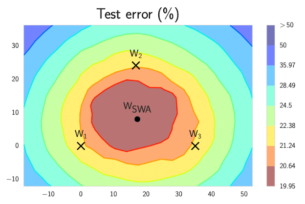
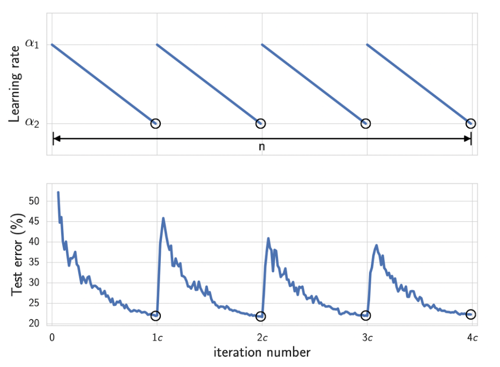
The explorations of the model weights around these flat regions of low loss is done by using a modified cyclic learning schedule that interpolates between large and small learning rates. The SGD optimizer uses these learning rates to jump around the basin when it is large, and sample model weights when the learning rate is low and has converged to some point on the flat low loss surface.
By doing this multiple times over separate training runs with different starting configurations and hyper-parameters, you can approximate many basins of attraction in the posterior of the weights. By taking samples of these weights from the mixture of gaussians and ensembling the different model’s predictions you can approximate the posterior and preform BMA, leading to much more accurate predictions that account for epistemic uncertainty.
INTERESTING RELATION TO AUDIO PROCESSING
The sequential estimation framework used in Project Skydrop shares a strong mathematical connection with the approach to Automatic Speech Recognition (ASR). For decades the industry standard for transcribing speech was the Hybrid Hidden Markov Model system. This solves a problem nearly identical to our treasure hunt which is inferring a hidden sequence of states (words) from a noisy stream of observations (audio).
MORE INFO
In the context of speech the goal is to find the most likely word sequence W given an audio signal A. This is decomposed using Bayes’ Rule into two components. These are the Language Model P(W) which acts as the prior and the Acoustic Model P(A|W) which acts as the likelihood.
In our geospatial search we perform the exact same decomposition. We combine a prior belief about the treasure’s location P(St) with the likelihood of seeing specific sensor data given that location P(Xt|St).
There is a critical difference in how we calculate that likelihood term. In modern speech recognition engineers often use a discriminative approach. Because neural networks are excellent at classification they train a model to predict the word given the audio P(W|A). They then mathematically invert it using Bayes’ rule to recover the likelihood needed for the HMM.
For Project Skydrop we deliberately reject this discriminative shortcut in favor of Direct Likelihood Estimation via Flow Matching. The reason lies in the fundamental nature of the mapping between our variables.
In speech the mapping from Audio to Word is many-to-one. Thousands of variations in pitch, accent, and speed all collapse into the single label “Cat”. A discriminative neural network excels here because it can learn to ignore the variance and confidently predict the single correct class.
In our treasure hunt the mapping from Data to Location is one-to-many. A single temperature reading over a day doesn’t necessarily point to one location. It is consistent with many of the grid cells across the search area. This is a classic inverse problem. If we attempted to train a discriminative model P(St|Xt) to predict the location based on temperature the output distribution would be incredibly flat or prone to mode collapse. The network struggles to distribute probability mass across disparate regions of the map.
By using Flow Matching to model the generative direction P(Xt|St) directly we align our model with the causality of the physical world. While it is hard to guess a location given a temperature it is straightforward to predict the temperature given a location and satellite context.
By solving the forward physics rather than the inverse classification our model remains robust in a low-data regime. It learns the universal relationship between satellite maps and ground sensors which holds true everywhere rather than attempting to memorize the unique thermal signature of every specific grid cell.
CONCLUSION
The results are calibrated likelihoods for where the hidden location is located. I built a web application to visualize the progression of the HMM through the days of simulated treasure hunts on real held out data.
References:
- E. Hüllermeier and W. Waegeman, “Aleatoric and epistemic uncertainty in machine learning: an introduction to concepts and methods,” Machine Learning, vol. 110, no. 3, pp. 457–506, 2021. Available: https://link.springer.com/article/10.1007/s10994-021-05946-3
- P. Izmailov, D. Podoprikhin, T. Garipov, D. Vetrov, and A. G. Wilson, “Averaging weights leads to wider optima and better generalization,” arXiv preprint arXiv:1803.05407, 2018. Available: https://arxiv.org/abs/1803.05407
- A. Kendall and Y. Gal, “What uncertainties do we need in Bayesian deep learning for computer vision?” arXiv preprint arXiv:1703.04977, 2017. Available: https://arxiv.org/abs/1703.04977
- W. Maddox, T. Garipov, P. Izmailov, D. Vetrov, and A. G. Wilson, “A simple baseline for Bayesian uncertainty in deep learning,” arXiv preprint arXiv:1902.02476, 2019. Available: https://arxiv.org/abs/1902.02476
- J. Rohrer and T. Bailey, “Project SKYDROP,” 2024. [Online]. Available: https://projectskydrop.com/
- O. Rybkin, K. Daniilidis, and S. Levine, “Simple and Effective VAE Training with Calibrated Decoders,” arXiv preprint arXiv:2006.13202, 2020. Available: https://arxiv.org/abs/2006.13202
- M. Schofield, “Project Skydrop treasure found in Wendell State Forest,” The Greenfield Recorder, 2024. [Online]. Available: https://www.recorder.com/Project-Skydrop-treasure-found-in-Wendell-State-Forest-57285704
- J. S. Speagle, “A conceptual introduction to Markov Chain Monte Carlo methods,” arXiv preprint arXiv:1909.12313, 2020. Available: https://arxiv.org/abs/1909.12313
- A. G. Wilson and P. Izmailov, “Bayesian deep learning and a probabilistic perspective of generalization,” arXiv preprint arXiv:2002.08791, 2020. Available: https://arxiv.org/abs/2002.08791
