Distributed Cloud Computing for Machine Learning

Tags: FSDP, Google Cloud Platform, PyTorch, Spark

OVERVIEW

The goal of this project is to understand how modern deep learning frameworks scale training across multiple devices. Rather than treating distributed training as a black box, this project focuses on the underlying principles that make large-scale learning possible, such as parallelism, communication, and synchronization. To explore these ideas in practice, I implement a custom distributed machine learning algorithm using the Spark framework, applying the same core concepts that appear in distributed ML systems within a more general-purpose distributed computing environment.

WHY WE NEED TO SCALE

The need to scale arises from an increased demand for computational abilities for some application beyond the capabilities of a single device. This is often handled through either vertical or horizontal scaling. Vertical scaling is trying to upgrade or increase the computational resources of your single device, while horizontal scaling focuses more on increasing the number of devices able to be used for computation.

While horizontal scaling does require more complex coordination between devices, its benefit is that its much easier and cheaper to just add more devices to a computing cluster, rather than trying to spend loads of money on the latest super computer, which hits a computational limit much faster than simply adding more devices. We focus on horizontal scaling for these reasons under the specific assumptions of supporting the scaling of deep neural networks.

There are two main reasons why a data processing application would need to scale.

One is purely the amount of data that is available to process. Where a single device would just take forever to preform the necessary computations.
The other is the size of the data processing algorithm. Especially in modern deep neural networks the computation model size can grow to be far too large to sit on a single device and needs to be distributed among many devices to even be able to pass any data through.

TYPES OF PARALLELISM

Data parallelism: Solves the first of these issues where there is just too much data. It does this by replicating the model across each device in the cluster. That way each device can process its own batch of data independently, speeding up the data throughput of the neural network. After the forward pass, all of these separate devices now need to share gradient information from their respective passes such that an update to the network’s parameters can be preformed across all devices. In practice, the communication of gradients is done concurrently as soon as the model’s forward pass has gotten far enough for a chunk of gradients to be aggregated. This technique of course assumes that the network parameters and gradients can fit entirely on a single device, and can thus be replicated across the cluster.

Model parallelism: Takes a slightly different approach in order to solve the second problem of networks being so large they can’t fit on a single device. This is typically done by constructing a model pipeline where each device, claims ownership of specific layers of the network. The different devices are then arranged sequentially such that a full forward pass can be computed distributed across the devices, where one device passes its layer’s output to the next.

COMMUNICATION PRIMITIVES

Communication primitives are the underlying methods in which data is shared across the computing cluster in an efficient way. Lets first define some key terms that will help with the understanding of the process:

Rank: This is a process that has access to a single GPU. Ranks can exist on the same physical computer or can be distributed across clusters.
Layers: This is what makes up the computational graph of the neural network. Each layer passes it’s output to the next and needs to be preformed sequentially.
Units: This is a collection of layers. Typically for very large model’s the layers are split up into units such that each can fit fully in a rank’s memory.
Shard: This is a subset of a unit’s parameters or gradients that is typically owned by a specific rank.

There are three main communication primitives.

All-Reduce: Takes data that is distributed across the computing cluster and aggregates it together (sums or averages). It then ensures that each rank in the cluster has a copy of this fully reduced data.

Reduce-Scatter: Takes data that is distributed across the computing cluster and aggregates it together, leaving the reduced copies scattered across ranks in the computing cluster.

All-Gather: Takes data that is scattered across the computing cluster and ensures that each rank has a complete copy of this data.

You can think of the All-Reduce primitive as being a Reduce-Scatter immediately followed by an All-Gather, such that the data is both reduced and gathered on all ranks. In some algorithms for these primitives (ring algorithm), it actually follows this decomposition.

The ring algorithm arranges ranks in a ring, where each rank only communicates with its neighbors. The communication primitives above are implemented under this type of communication structure. The main benefits of this structure are…

Bandwidth optimal: Meaning that each rank sends the same amount of data between its neighbors, regardless of the cluster size.
No central bottleneck: Theres no master node in which communication depends on, the load is evenly split among all of the ranks.

Because of this bandwidth optimality the algorithm is really great for most deep learning applications, as the gradients that we are communicating are typically very large and the whole process is bandwidth bound.

The main drawback of this method is the linear scaling of compute latency, since the data has to pass through the entire ring structure. Thats where other options like the tree algorithm come into play.

The tree algorithm works by arranging ranks into a tree structure such that the parent communicates with all child ranks and each child rank communicates with it’s parent. In this way we can achieve logarithmic latency in these communication primitives, at the cost of a potentially uneven distribution of communication load across ranks (not bandwidth optimal).

Typically the tree alogorithm is used in very large compute clusters where latency is the concerning factor over bandwidth. In practice these algorithms are often combined for specific computing use cases.

Because typical applications are bandwidth bound we will examine the ring algorithm in greater detail.

Ring Reduce-Scatter:

For this example lets assume we have 4 ranks, where each rank holds some gradient data. Our first step is to chunk up this data that we want to reduce into rank number of chunks.

Each rank takes reducing responsibility for one chunk, that way the results remain scattered at the end. In each step of this process a rank sends all other chunks they are not responsible for to their neighboring rank. The neighboring chunk takes in those passed along chunks, accumulating the chunk its responsible for while storing the rest to be passed on in the next iteration.

The algorithm repeats this process until each rank holds a fully reduced version of the chunk its responsible for. At this point the gradients are reduced (summed up) and scattered across the different ranks.

For Data Parallel distributed systems you ideally want the reduced gradient chunks to not be scattered but exist on all machines in full. Its possible to use the ring algorithm to reduce across all chunks at once, resulting in a non scattered fully reduced gradient on each rank. However in order to support this each rank would need to use twice the memory for the gradients, one for accumulating gradients and another for passing the partial gradients of the prev neighbor to the next rank in the ring. Rather than using up more memory, what is typically done is that a reduce-scatter is immediately followed by a all-gather, to result in fully reduced gradients on each machine, without requiring extra memory.

Ring All-Gather:

This ring algorithm is conceptually simpler than the reducing one because all we are doing is passing data down the line of ranks until every rank has a copy of every other rank’s data.

As mentioned before, in data parallel systems the data chunks that we are gathering are typically already reduced gradients. With the goal being to get a full copy of the reduced gradients on each rank, so that a gradient update step to the parameters can be preformed in parallel.

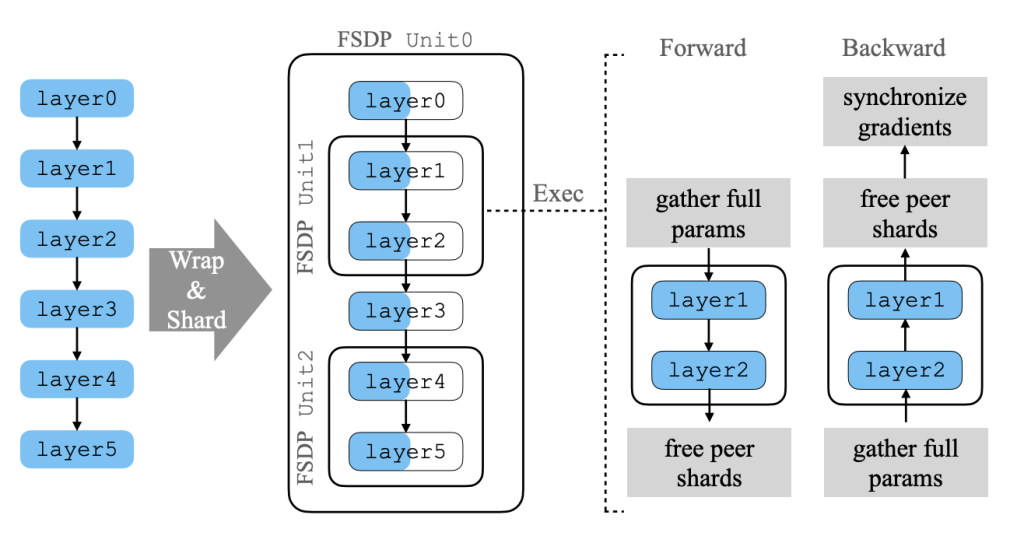
FULLY SHARDED DATA PARALLELISM

FSDP is similar to a combination of data and model parallelism techniques where you have this linear scaling of effective batch sizes with compute, along with the reduced model memory requirements of model pipelining. You are basically model pipelining but within a single rank, replicating that processes across all ranks. The reason you can model pipeline within just one rank rather than linking multiple ranks in sequence is because of model sharding, which splits up the memory requirements of the model across all of the ranks. In that way each rank only needs to gather the correct parameters to execute a forward/backward pass of one unit at a time.

An All-Gather operation is used to gather a specific unit’s parameters on each of the ranks such that those layers in the unit can be computed in parallel. After the rank is done with these parameters, they are discarded and it moves on to the next unit in the model pipeline. Typically the gathering of these parameters can be overlapped with the actual computation of the model, so there is not too much time waiting in between passes of the model.

In order to actually update the model weights you need to aggregate the gradient information across each of the ranks. Since the model weights are sharded and stored separately across all the ranks we want the reduced gradients to also remain sharded with the corresponding parameters so that the parameters can be updated in their sharded states. This means that we want to use a Reduce-Scatter operation such that these gradients remain distributed across the ranks.

The only real difference between pipelining within a single rank and across multiple ranks is that since a single rank computes the entire model pipeline, it needs to store all intermediate activations such that the backwards pass can be preformed and gradients can be calculated. These activations can’t easily be sharded in the same way that parameters or gradients can because they are rank mini batch specific (they depend on the specific data that each rank was given). This differs from pipeline model parallelism because each rank there only needed to worry about the activations of it’s own layers and not of the entire model.

There are multiple strategies to deal with this increased memory requirement. Including activation checkpointing in between key layers of the model, such that a mini forward pass can be computed to recover fine grained activations between layers, saving memory. Another strategy is offloading these activations to the CPU and then doing prefetching to get back these activations during the backward pass.

OTHER TYPES OF DISTRIBUTED COMPUTATION

While this project focuses on distributed machine learning, the same core ideas of distributed computation appear in many other systems. One of the most widely used examples is Apache Spark, a framework designed for large-scale data processing. Spark is typically used when datasets are too large to fit on a single machine and need to be processed in parallel across a cluster. Common use cases include batch analytics, ETL pipelines, and large-scale statistical computations.

Spark approaches distributed computing very differently from modern ML frameworks. Instead of tightly synchronized workers and frequent communication, Spark favors coarse-grained parallelism and fault tolerance. Data is split into partitions, and computations are expressed as transformations that operate independently on each partition. If part of the computation fails, Spark can recompute results using lineage information rather than requiring strict synchronization between workers. This makes Spark well suited for high-throughput data processing, but poorly suited for low-latency numerical workloads like deep learning.

Despite these differences, there are clear conceptual parallels. Spark often performs distributed aggregation operations, where partial results are computed on each partition and then combined across the cluster. At a high level, this resembles communication patterns like Reduce or All-Reduce used in distributed ML. In Spark, these reductions are typically organized hierarchically and materialized on a central driver, which may then broadcast the result back to workers for use in later stages.

The key distinction is that Spark’s communication operates on serialized objects and dataset partitions, often involving disk and network shuffles, while ML frameworks operate directly on in-memory tensors with carefully optimized collective communication. As a result, Spark and distributed ML systems target very different applications, even though they rely on many of the same fundamental distributed computing principles.

SPARK DISTRIBUTED TRAINING

Since I don’t have access to multiple GPUs to experiment with distributed computation for ML, I chose to implement an ML algorithm within the Spark framework. While this is far from computationally efficient compared to GPU-based training, it still benefits from Spark’s core strengths: cheap horizontal scalability, built-in fault tolerance, and seamless integration with large-scale data preprocessing pipelines.

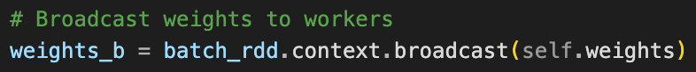
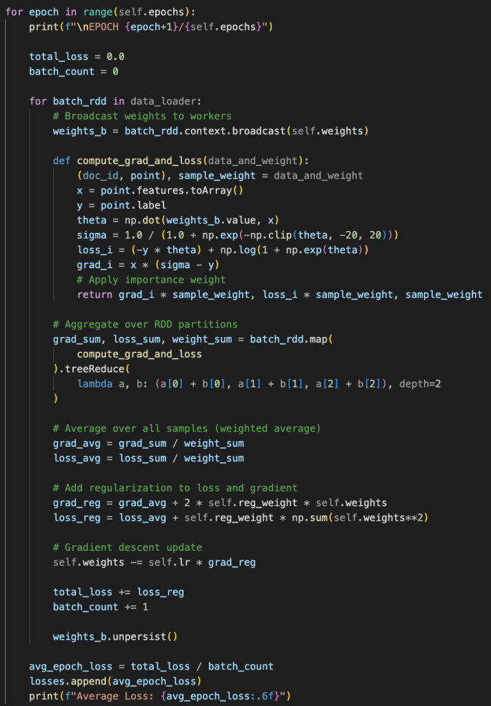
The model I implemented is a logistic regression document classifier trained using distributed gradient descent. Each Spark worker processes a subset of documents and independently computes loss and gradient contributions for its local data. This closely mirrors data parallel training in distributed ML systems, where each rank processes a different mini-batch using a shared set of model parameters. In this implementation, the current weights are broadcast from the driver to all workers at the start of each batch so that gradients are computed consistently across the cluster.

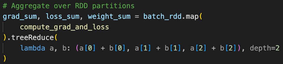
Once local gradients are computed, they must be aggregated to produce a global update. Spark performs this aggregation using a tree-structured reduction, where partial results are combined hierarchically before being returned to the driver. Modern ML frameworks use similar tree-based reductions in some settings for the same reason: reducing latency. A tree structure allows aggregation to complete in logarithmic time with respect to the number of workers, rather than requiring data to pass sequentially through all devices. While Spark’s reduction operates on serialized objects and ends on a central driver, the underlying motivation for the tree structure is shared.

After the aggregated gradient is computed, the driver performs the parameter update and broadcasts the updated weights back to the workers for the next iteration. Although this reduce-then-broadcast pattern is much slower than GPU-based collective communication, it demonstrates how the same distributed optimization principles apply across very different systems. Spark trades low-latency communication for robustness, scalability, and tight integration with data pipelines, making it a useful framework for exploring distributed learning ideas even outside of traditional ML training environments.

The distributed gradient decent optimization loop used in the training of the Spark logistic regression classifier.

CONCLUSION

This project examined how the core ideas behind distributed machine learning appear in practice by implementing a simple learning algorithm in Spark. Although Spark is not designed for low-latency numerical computation and is not competitive with GPU-based training frameworks, it provides a clear view into how distributed computation, aggregation, and synchronization work at scale. Comparing this approach with modern ML frameworks highlights the different design trade-offs between performance, fault tolerance, and system complexity. These trade-offs explain why distributed ML systems rely on specialized communication primitives, while general-purpose frameworks like Spark prioritize robustness and scalability over raw efficiency.