
OVERVIEW
Rendering realistic images is always a balance between accuracy and speed. If you’ve ever played a video game after seeing a rendered cinematic trailer and left less than impressed, you’ve seen this problem firsthand. This project is about tackling one of the big bottlenecks: getting clean, sharp images from path tracing without paying the huge cost of supersampling.
The idea is to use neural networks to help with anti-aliasing and denoising — letting us keep the realism of path tracing while cutting down on the number of rays we need to shoot. I use a custom built path tracing algorithm to fully test and analyze this possibility. But before diving into how that works, let’s take a step back and walk through the basics.
- PHYSICALLY BASED RENDERING
- RAY TRACING
- PATH TRACING
- ISSUE: ANTI-ALIASING
- ISSUE: SAMPLING NOISE
- EARLY ATTEMPTS AT A NEURAL NETWORK
- STABLE DIFFUSION
- STABLE SR
- CONCLUSION
PHYSICALLY BASED RENDERING
Physically based rendering (PBR) is all about simulating how light actually behaves. Instead of just faking lighting with tricks, we try to model the physics of light bouncing around a scene and into the camera. This means that as we pay more attention to the underlying process of the real world, things like color bleeding between surfaces, soft shadows, glossy reflections, and light refracting through glass naturally follows from the simulation process.
This is different from rasterization — what most game engines still use — which is built for speed and approximation. Rasterization is great for real-time applications, but it struggles to match the realism that PBR achieves, and often involves highly engineered algorithms to account for this.
A key part of PBR is the BRDF (Bidirectional Reflectance Distribution Function), which basically describes how light scatters off a material. Combine BRDFs with algorithms like ray tracing and path tracing, and you get increasingly physically accurate images… but at a cost of runtime.
RAY TRACING
Ray tracing starts simple: shoot a ray from the camera through each pixel into the scene, figure out what it hits, and then work out the color of that hit point. To figure out lighting, you might spawn secondary rays — shadow rays toward light sources, reflection rays for shiny surfaces, refraction rays for glass, etc.
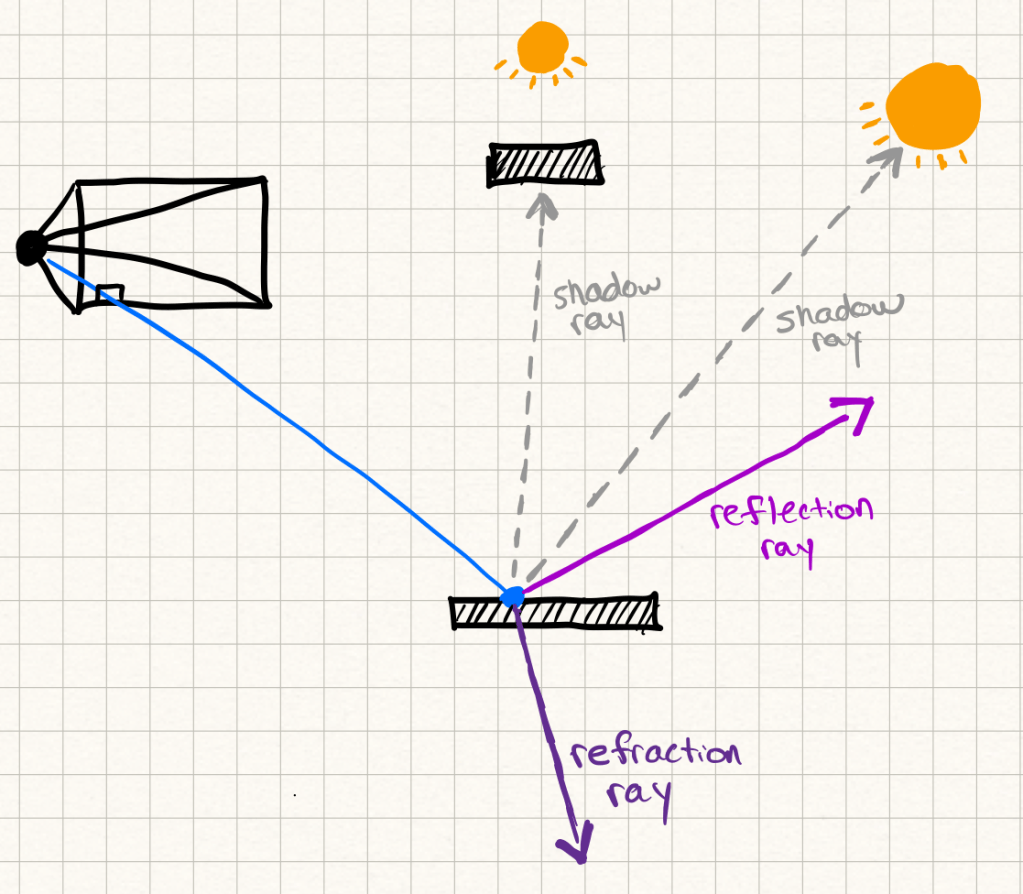
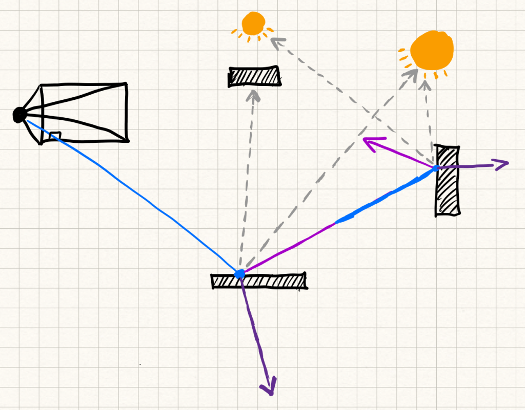
The process can recurse deeper and deeper as rays keep bouncing. In practice, you usually set a maximum depth, otherwise the number of rays explodes. Usually after a couple recursions the light contributions of new rays diminish and you are better off saving the runtime.
Ray tracing gives you accurate direct lighting, sharp reflections, and defined shadows, but still has limitations. It doesn’t naturally capture more complex effects like indirect lighting or soft shadows without adding more complexity. For each ray cast secondary rays imitate how light could have reached that point without actually modeling the scattering of rays on the surface. That’s where path tracing comes in.
PATH TRACING
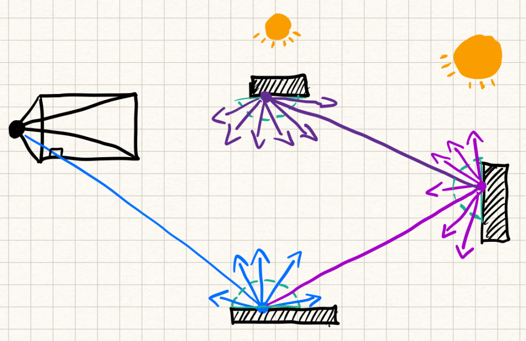
Path tracing is like ray tracing, but instead of carefully picking which rays to spawn, it takes a Monte Carlo approach at approximating the scattering of rays on the object’s surface. At each surface hit, you sample a direction from the hemisphere above the surface, and send the ray off in that direction.
The true solution would be to integrate over the entire hemisphere of possible scattering directions. That’s intractable, so path tracing approximates it with random samples. Instead of doing recursive hemisphere sampling, it usually samples entire trajectories — full random paths of rays bouncing through the scene.
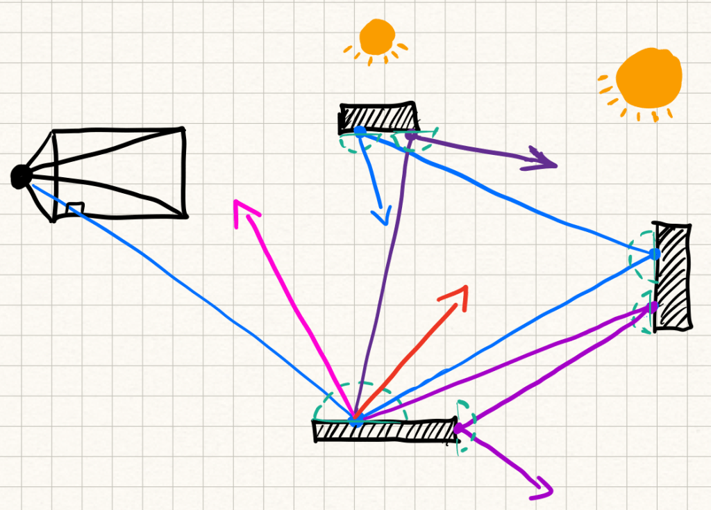
To keep things unbiased but still manageable, path tracers use techniques like Russian roulette. After a certain number of bounces, each ray has a probability of being terminated. This cuts down the average path length while still giving the right result in expectation.
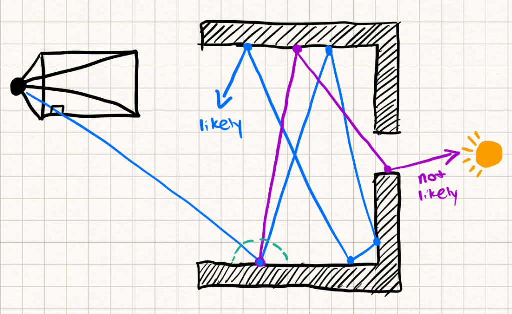
The big issue here is variance. Imagine a scene where the only light source is behind a small window. Most rays will never make it to the light, so the few that do will have high variance and create noise in the image.
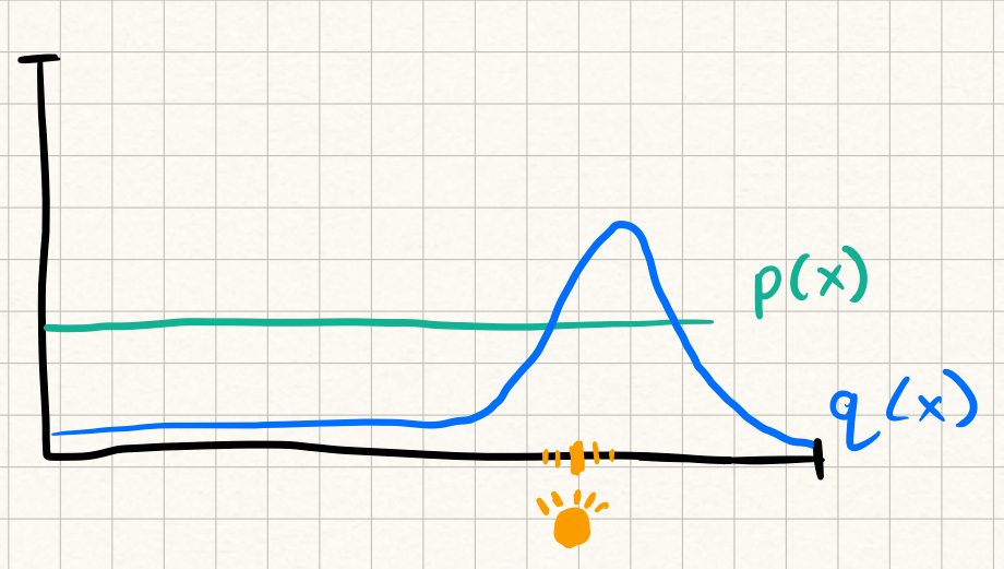
Importance sampling helps. Instead of sampling uniformly across the hemisphere, you bias your samples toward directions that are likely to contribute more — like pointing rays toward the light source. Here p(x) is the uniform distribution we usually sample from on the hemisphere. When sampling from p(x) most of the samples will have very little light contribution. But by sampling from the proposal distribution q(x) and reweighing the result we can encourage more rays to reach the light, while remaining unbiased.
This reduces variance, but it doesn’t eliminate noise. Even with importance sampling, path tracing takes a ton of rays to converge to a clean image.
ISSUE: ANTI-ALIASING
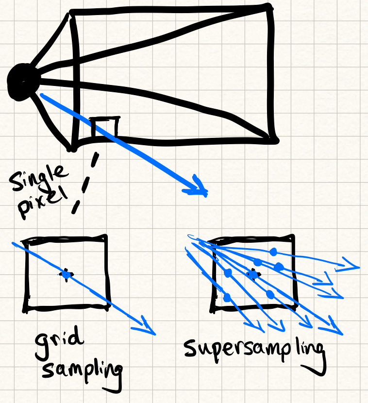
On top of sampling noise, there’s also the problem of aliasing. Aliasing shows up as jagged edges when thin geometry is under sampled on the pixel grid.
The brute force solution is supersampling: shoot multiple rays per pixel, slightly jittered, and average them together.
This works beautifully but is expensive, since each extra ray multiplies your compute cost.
Here’s where neural networks start to get interesting. Instead of just firing more rays, you can train a model to recognize and smooth out aliasing artifacts. A network can learn the difference between a true edge and a sampling artifact, and reconstruct a cleaner pixel grid from fewer rays.
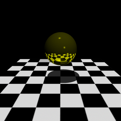
The examples below show some of the results before and after using a neural network to correct a render’s low sample aliasing artifacts.


Right: StableSR Render
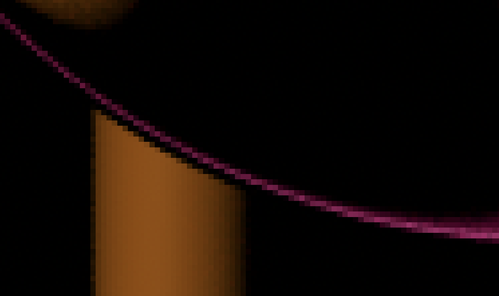
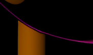
Right: StableSR render
ISSUE: SAMPLING NOISE
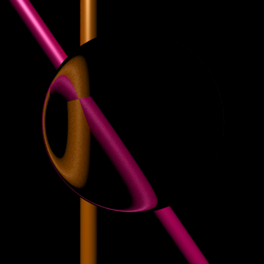
As mentioned before Monte Carlo noise is the other big problem in path tracing. You see it as speckles, especially in tricky situations like caustics (light focusing through glass or water), deep shadows, or scenes with difficult to reach light sources.
The obvious fix is, again, more samples per pixel. But doubling the number of rays doesn’t halve the noise — it only reduces it by the square root of the sample count. That’s an expensive tradeoff.
A simple trick is to apply a Gaussian filter across the image, which averages nearby pixels together. This smooths out noise, but it also smears edges and destroys fine details.
Neural networks can do better. Because they’re trained on real images, they develop priors about what edges and textures should look like. Instead of just smoothing, they can selectively denoise — removing random speckles while keeping high-frequency detail intact. That means thin lines, crisp edges, and fine textures survive the process.
Models like StableSR use this idea: they can clean up path-traced noise in a way that still respects the underlying structure of the scene. This lets us get to a visually clean render much faster, without brute-forcing millions of rays.
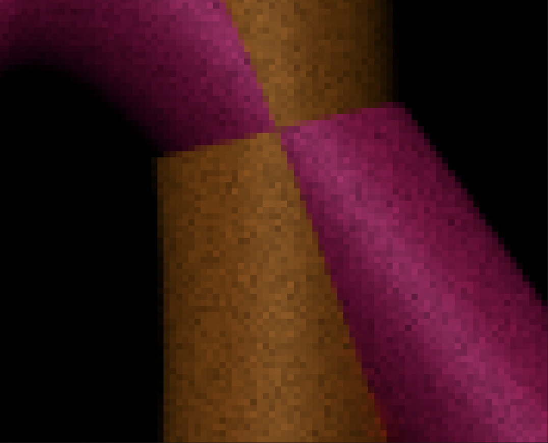
Bottom: StableSR render
EARLY ATTEMPTS AT A NEURAL NETWORK
My initial goal was to train a lightweight neural network that could recognize and correct rendering artifacts directly within my ray and path tracing pipeline. The first challenge was data. There weren’t any public datasets pairing low-sample renders with their high-quality, supersampled versions. Ideally, I would have generated my own dataset by producing a wide range of 3D scenes at multiple sample rates, but the rendering time required made that approach unrealistic.
Instead, I tried working backward. Rather than start with noisy renders, I took clean images from the web and artificially degraded them to simulate under-sampling. The idea was simple: by training a model to restore these degraded images to their sharp originals, it might learn priors that could transfer to real path-traced noise. In practice, though, the model learned to handle only the specific kinds of degradation I introduced — things like bicubic downsampling and Gaussian blur — rather than the structured noise patterns that appear in physically based rendering.
To bridge that gap, I had two options: dramatically expand my dataset or leverage an existing model with a richer learned prior about natural images. This led me to diffusion models, and specifically Stable Diffusion, as a foundation to explore.
STABLE DIFFUSION
Stable Diffusion, developed by Stability AI, is an open-source text-to-image model that generates realistic visuals through an iterative denoising process known as diffusion.
In essence, the model works in latent space, a compressed representation of images created by a variational autoencoder (VAE). Starting from random noise, the diffusion model gradually refines its latent representation toward regions of higher probability that correspond to real images. The result is an image that reflects the model’s learned understanding of structure, texture, and realism.
The real strength of Stable Diffusion lies in these priors—the immense amount of visual knowledge captured from training on large datasets. The challenge is using those priors to enhance a rendered image without letting the model change it too much. We want it to fix artifacts, not reinterpret the scene.
This control happens through conditioning. In text-to-image generation, the U-Net uses cross-attention layers to align image features with semantic cues from text embeddings. Modifying these attention mechanisms directly is costly and can destabilize the learned generative prior we want to keep intact.
That’s what makes StableSR interesting. It offers a way to perform super-resolution using diffusion priors while keeping the base model frozen and stable.
STABLE SR
The StableSR model, developed by Jianyi Wang, is from the paper: Exploiting Diffusion Prior for Real-World Image Super-Resolution.
Super-Resolution
This paper makes three main contributions which allow the super resolution of images utilizing the diffusion prior with as little trainable parameters as possible.
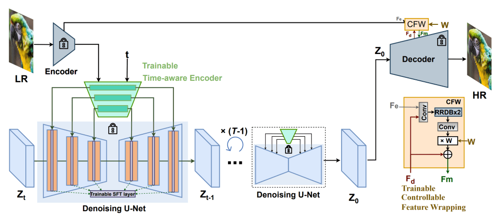
- Time-Aware LR Encoder
A small CNN extracts multi-scale features from the low-resolution latent image. It also takes in the current diffusion timestep, allowing it to adapt its output as the process unfolds. Early in denoising, the U-Net benefits from stronger guidance that preserves global structure; later, the encoder eases off to let the diffusion model fill in fine details. - Spatial Feature Transform (SFT) Modulation
SFT layers provide non invasive, low parameter count alternatives to cross attention. They use scale and shift parameters derived from the LR encoder to modulate intermediate feature maps in the U-Net. You can think of it as at each feature position, you emphasize or suppress features according to this external conditioning. This lets the model stay aligned with the low-resolution input while still taking advantage of the pre-trained diffusion prior. - Controllable Feature Wrapping Module
The final component blends the outputs of the original LR latent and the diffusion-refined latent. A tunable weight between 0 and 1 controls the tradeoff between fidelity to the input and the realism introduced by the diffusion prior. During training, this module uses a small CNN with perceptual and adversarial losses to learn to balance detail and consistency.
Together, these modules allow StableSR to super-resolve images by tapping into the learned structure of diffusion models without retraining the full network.
CONCLUSION
Path tracing gives us a physically accurate foundation for realistic lighting and material behavior. It captures the way light actually moves through a scene, producing results that feel grounded in the real world. The tradeoff, as always, is efficiency — getting that level of realism requires a huge number of samples.
Diffusion models help close that gap. They bring learned priors from real images that can smooth noise, sharpen edges, and restore detail without the heavy cost of additional ray samples. Instead of relying purely on simulation, they draw on statistical knowledge of what natural images should look like.
Together, these methods point toward a hybrid rendering scheme: physics providing the structure and realism, and neural networks providing the efficiency.
